Basic Hydrodynamic Equations
With increasing urbanization and urban renewal impacts driving the drainage and water quality regulatory framework, the design and analysis of storm water systems are becoming increasingly complex. The hydraulics characteristics of a drainage system often exhibit many complicated features, such as tidal or other hydraulic obstructions influencing backwater at the downstream discharge location, confluence interactions at junctions of a pipe network, interchanges between surcharged pressure flow and gravity flow conditions, street-flooding from over-loaded pipes, integrated detention storage, bifurcated pipe networks, and various inline and offline hydraulic structures. The time variations of the storm drainage design flow event are increasingly important in verifying total performance and achieving a measure of regulatory or design policy compliance. To better understand these complicated hydraulic features and accurately simulate flows in a complicated storm water handling system hydrodynamic flow models are necessary.
To simulate unsteady flows in storm water collection systems, numerical computational techniques have been the primary tools, and the results from numerical models are widely used for planning, designing and operational purposes. Since an urban drainage system can be composed of hundreds of pipes and many hydraulic control structures, the hydraulics in storm system can exhibit very complicated flow conditions. Consequently the numerical stability, computational performance, capabilities and robustness in handling complicated hydraulic conditions and computational accuracy are the major factors when deciding which approach to use to solve the hydraulic system.
Although many numerical methods have been developed to simulate the unsteady flows in sewer and storm water systems, including those based on explicit numerical schemes and those based on implicit schemes, limitations in most of models exist. Drainage and Utilities features engines capable of solving the dynamic solution using both schemes. Users may select to either user EPA SWMM’s native explicit solver or a custom implicit solver as more fully described in this section. The implicit solver is the default solver used in Drainage and Utilities.
Flows in sewers are usually free surface open-channel flows, therefore the Saint-Venant equations of one-dimensional unsteady flow in non-prismatic channels or conduits are the basic equations for unsteady sewer flows. The dynamic model solution uses the following complete and extended equations:
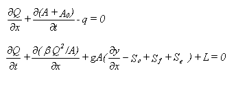
| t | = | time | |
| x | = | the distance along the longitudinal axis of the sewer reach | |
| y | = | flow-depth | |
| A | = | the active cross-sectional area of flow | |
| A 0 | = | the inactive (off-channel storage) cross-sectional area of flow | |
| q | = | lateral inflow or outflow | |
| â | = | the coefficient for nonuniform velocity distribution within the cross section | |
| g | = | gravity constant | |
| S o | = | sewer or channel slope | |
| S f | = | friction slope due to boundary turbulent shear stress and determined by Manning’s equation | |
| S e | = | slope due to local severe expansion-contraction effects (large eddy loss) | |
| L | = | the momentum effect of lateral flow |
Equation 14.1 is known as continuity equation and equation 14.2 is known as momentum equation. The two equations represent a complete unsteady flow hydrodynamic equation system therefore a dynamic model based on them is known as dynamic routing model or dynamic model.
Sometimes simplified equations, by neglecting a few terms in the momentum equation, are used in a model and the model becomes kinematic or diffusion model depending on what terms are neglected. This will be further discussed in the special consideration section.